FLIM Data analysis

Code blocks for FLIM data phasor analysis

First, we try to load some calibration fluorophore of known lifetime (Rhodamine B, Erytrosine B and the mixture) and visulize them in the phasor plot:

# Import necessary packeges
import numpy as np
from sdtfile import SdtFile
import matplotlib.pyplot as plt

# Select the sdt file
file_path = "./static/sdt/calibration/rhodamineB_in-methanol_ex805_1024x1024_px180_em610_05AOM_05_internal_001.sdt"
# Load the sdt file and print the number of channels
flim_file = SdtFile(file_path)
print("The number of channels is: ", len(flim_file.data))
# Load the data from first channel
data = flim_file.data[0]
print("The shape of the data is (x, y, time bins): ", data.shape)

The number of channels is:  1
The shape of the data is (x, y, time bins):  (1024, 1024, 256)

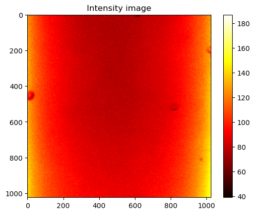
# Create an intensity image of the FLIM data and plot it
intensity_image = np.sum(data, axis=2)
# Plot the intensity image
plt.imshow(intensity_image, cmap='hot')
# Add colorbar
plt.colorbar()
# Add title
plt.title("Intensity image")
plt.show()

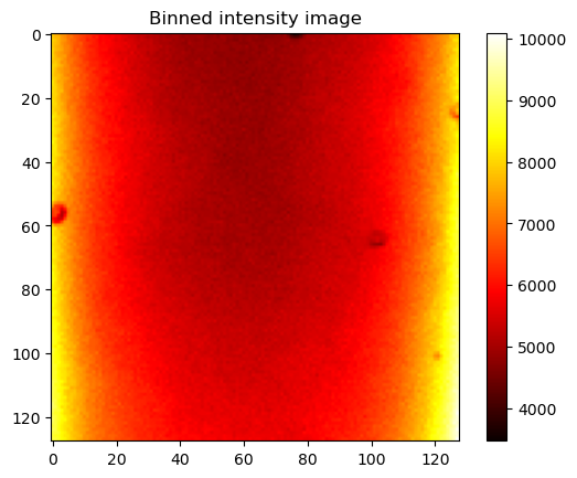
# Bin the data in x, y to increase the photon count
# Bin factor
bin_factor = 8
# Bin the data according to the bin factor
binned_image = intensity_image.reshape((intensity_image.shape[0] // bin_factor, bin_factor,
                                  intensity_image.shape[1] // bin_factor, bin_factor)).sum(axis=(1, 3))
# Plot the binned image
plt.imshow(binned_image, cmap='hot')
plt.colorbar()
plt.title("Binned intensity image")
plt.show()

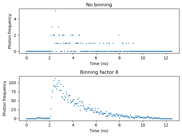
# Plot the flourescence lifetime decay for a pixel and binned data
# Create a time array for the x-axis
time = np.linspace(0, 12.5, data.shape[2])
# Binned data according to the bin factor and keep the third dimension
data_binned = data.reshape((data.shape[0] // bin_factor, bin_factor,
                            data.shape[1] // bin_factor, bin_factor,
                            data.shape[2])).sum(axis=(1, 3))
# Select a pixel from the data with all the time bins
data_pixel = data[512, 512, :]
# Select a pixel from the binned data
data_binned_pixel = data_binned[512 // bin_factor, 512 // bin_factor, :]
# Plot the results
fig, ax = plt.subplots(2, 1)
ax[0].scatter(time, data_pixel, s = 2)
ax[0].set_title("No binning")
ax[0].set_xlabel("Time (ns)"), ax[0].set_ylabel("Photon frequency")
ax[1].scatter(time, data_binned_pixel, s = 2)
# ax[1].set_yscale("log")
ax[1].set_title("Binning factor " + str(bin_factor))
ax[1].set_xlabel("Time (ns)"), ax[1].set_ylabel("Photon frequency")
fig.tight_layout() 

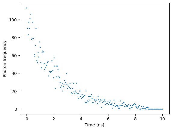
# Find the index of the maximum value in decay data
max_index = np.argmax(data_binned_pixel)

# Slice the vector to keep only the values on the right side behind the peak
sliced_data = data_binned_pixel[max_index:]
sliced_time = time[max_index:]
sliced_time = sliced_time - sliced_time[0]

# Plot the sliced data
plt.scatter(sliced_time, sliced_data, s = 2)
plt.xlabel("Time (ns)"), plt.ylabel("Photon frequency")
plt.show()

# Laser frequency input
f_laser = 80e6
omega = 2 * np.pi * f_laser

# Time vector
t = sliced_time*1e-9

# Calculate the phasor coordinates
g = np.sum(sliced_data * np.cos(omega * t)) / np.sum(sliced_data)
s = np.sum(sliced_data * np.sin(omega * t)) / np.sum(sliced_data)

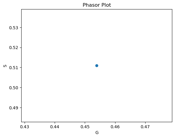
# Plot the phasor plot
fig, ax = plt.subplots(1,1)
ax.scatter(g, s, s=35)
ax.set_xlabel('G')
ax.set_ylabel('S')
ax.set_title('Phasor Plot')
plt.show()

# Plot the universal circle 
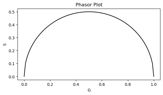
center_x = 0.5
center_y = 0
radius = 0.5
x_corr = np.linspace(-radius + center_x, radius + center_x, 100)
y_corr = radius * np.sqrt(1 - ((x_corr - center_x) / radius) ** 2) + center_y
fig, ax = plt.subplots(1,1)
ax.plot(x_corr, y_corr, 'k')
ax.set_xlabel('G')
ax.set_ylabel('S')
ax.set_title('Phasor Plot')
ax.axes.set_aspect('equal')

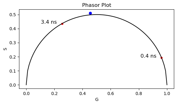
# Add the bound (3.4 ns) and free (0.4) NADH points to the phasor plot
tau = [3.4, 0.4]
g_NADH = []
s_NADH = []
# Calculate the phasor coordinates for the NADH points
for tau_m in tau: 
    s_now = (2*np.pi*f_laser*tau_m*1e-9)/(1 + (2*np.pi*f_laser)**2*((tau_m*1e-9)**2))
    g_now = 1/(1 + (2*np.pi*f_laser)**2*((tau_m*1e-9)**2))
    g_NADH.append(g_now)
    s_NADH.append(s_now)
NADH = np.vstack((g_NADH, s_NADH))
# Plot the phasor plot with the NADH points
fig, ax = plt.subplots(1,1)
ax.scatter(g, s, s = 35, c='b')
ax.plot(x_corr, y_corr, 'k')
ax.scatter(g_NADH, s_NADH, s=15, c='r')
ax.set_xlabel('G')
ax.set_ylabel('S')
ax.set_title('Phasor Plot')
# Plot text in x, y coordinates
ax.text(g_NADH[0]-0.15, s_NADH[0], '3.4 ns', color='k', fontsize=12)
ax.text(g_NADH[1]-0.15, s_NADH[1], '0.4 ns', color='k', fontsize=12)
ax.axes.set_aspect('equal')
# According to the literature, the Rhodamine B has a lifetime of ~ 2.2 ns.

# Calculate the phasor coordinates for all the point in the image
g_all = []
s_all = []

for idx_x in range(data_binned.shape[0]):
    for idx_y in range(data_binned.shape[1]):
        pixel_decay = data_binned[idx_x, idx_y, :]
        # Find the index of the maximum value in decay data
        max_index = np.argmax(pixel_decay)   
        # Slice the vector to keep only the values on the right side behind the peak
        sliced_data = pixel_decay[max_index:]
        sliced_time = time[max_index:]
        sliced_time = sliced_time - sliced_time[0]
        # Time vector
        t = sliced_time*1e-9
        g = np.sum(sliced_data * np.cos(omega * t)) / np.sum(sliced_data)
        s = np.sum(sliced_data * np.sin(omega * t)) / np.sum(sliced_data)
        g_all.append(g)
        s_all.append(s)
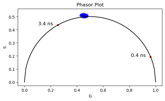
# Plot the phasor plot with the NADH points
fig, ax = plt.subplots(1,1)
ax.scatter(g_all, s_all, s = 2, c='b', alpha=0.1)
ax.plot(x_corr, y_corr, 'k')
ax.scatter(g_NADH, s_NADH, s=15, c='r')
ax.set_xlabel('G')
ax.set_ylabel('S')
ax.set_title('Phasor Plot')
# Plot text in x, y coordinates
ax.text(g_NADH[0]-0.15, s_NADH[0], '3.4 ns', color='k', fontsize=12)
ax.text(g_NADH[1]-0.15, s_NADH[1], '0.4 ns', color='k', fontsize=12)
ax.axes.set_aspect('equal') 

# Load erytrosine B data and plot the monoexponential decay in phasor
# Select the sdt file
file_path = "./static/sdt/calibration/erytrosineB_in-methanol_ex750_1024x1024_px180_em610_10AOM_10_internal_001.sdt"
# Load the sdt file and print the number of channels
flim_file = SdtFile(file_path)
print("The number of channels is: ", len(flim_file.data))
# Load the data from first channel
data = flim_file.data[0]
print("The shape of the data is (x, y, time bins): ", data.shape)

The number of channels is:  1
The shape of the data is (x, y, time bins):  (1024, 1024, 256)

# Plot the flourescence lifetime decay for a pixel and binned data
# Create a time array for the x-axis
time = np.linspace(0, 12.5, data.shape[2])
# Binned data according to the bin factor and keep the third dimension
data_binned = data.reshape((data.shape[0] // bin_factor, bin_factor,
                            data.shape[1] // bin_factor, bin_factor,
                            data.shape[2])).sum(axis=(1, 3))
# Calculate the phasor coordinates for all the point in the image
g1_all = []
s1_all = []

for idx_x in range(data_binned.shape[0]):
    for idx_y in range(data_binned.shape[1]):
        pixel_decay = data_binned[idx_x, idx_y, :]
        # Find the index of the maximum value in decay data
        max_index = np.argmax(pixel_decay)   
        # Slice the vector to keep only the values on the right side behind the peak
        sliced_data = pixel_decay[max_index:]
        sliced_time = time[max_index:]
        sliced_time = sliced_time - sliced_time[0]
        # Time vector
        t = sliced_time*1e-9
        g = np.sum(sliced_data * np.cos(omega * t)) / np.sum(sliced_data)
        s = np.sum(sliced_data * np.sin(omega * t)) / np.sum(sliced_data)
        g1_all.append(g)
        s1_all.append(s)
# Plot the phasor plot with the NADH points
fig, ax = plt.subplots(1,1)
ax.scatter(g1_all, s1_all, s = 2, c='b', alpha=0.1)
ax.scatter(g_all, s_all, s = 2, c='g', alpha=0.1)
ax.plot(x_corr, y_corr, 'k')
ax.scatter(g_NADH, s_NADH, s=15, c='r')
ax.set_xlabel('G')
ax.set_ylabel('S')
ax.set_title('Phasor Plot')
# Plot text in x, y coordinates
ax.text(g_NADH[0]-0.15, s_NADH[0], '3.4 ns', color='k', fontsize=12)
ax.text(g_NADH[1]-0.15, s_NADH[1], '0.4 ns', color='k', fontsize=12)
ax.axes.set_aspect('equal')
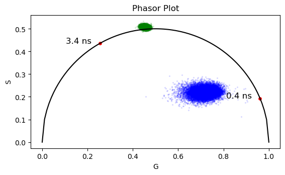
# According to the literature, the Erythrosin B has a lifetime of ~ 0.48 ns. 

# Mixture of rhodamineB(10%) and erytrosineB(90%) in methanol
# Load erytrosine B data and plot the monoexponential decay in phasor
# Select the sdt file
file_path = "./static/sdt/calibration/rhodamineB(1)+erytrosineB(9)_in-methanol_ex750_1024x1024_px180_em610_10AOM_10_internal_001.sdt"
# Load the sdt file and print the number of channels
flim_file = SdtFile(file_path)
print("The number of channels is: ", len(flim_file.data))
# Load the data from first channel
data = flim_file.data[0]
print("The shape of the data is (x, y, time bins): ", data.shape)
# Plot the flourescence lifetime decay for a pixel and binned data
# Create a time array for the x-axis
time = np.linspace(0, 12.5, data.shape[2])
# Binned data according to the bin factor and keep the third dimension
data_binned = data.reshape((data.shape[0] // bin_factor, bin_factor,
                            data.shape[1] // bin_factor, bin_factor,
                            data.shape[2])).sum(axis=(1, 3))
# Calculate the phasor coordinates for all the point in the image
g2_all = []
s2_all = []

for idx_x in range(data_binned.shape[0]):
    for idx_y in range(data_binned.shape[1]):
        pixel_decay = data_binned[idx_x, idx_y, :]
        # Find the index of the maximum value in decay data
        max_index = np.argmax(pixel_decay)   
        # Slice the vector to keep only the values on the right side behind the peak
        sliced_data = pixel_decay[max_index:]
        sliced_time = time[max_index:]
        sliced_time = sliced_time - sliced_time[0]
        # Time vector
        t = sliced_time*1e-9
        g = np.sum(sliced_data * np.cos(omega * t)) / np.sum(sliced_data)
        s = np.sum(sliced_data * np.sin(omega * t)) / np.sum(sliced_data)
        g2_all.append(g)
        s2_all.append(s)
# Plot the phasor plot with the NADH points
fig, ax = plt.subplots(1,1)
ax.scatter(g1_all, s1_all, s = 2, c='b', alpha=0.1)
ax.scatter(g_all, s_all, s = 2, c='g', alpha=0.1)
ax.scatter(g2_all, s2_all, s = 2, c='c', alpha=0.1)
ax.plot(x_corr, y_corr, 'k')
ax.scatter(g_NADH, s_NADH, s=15, c='r')
ax.set_xlabel('G')
ax.set_ylabel('S')
ax.set_title('Phasor Plot')
# Plot text in x, y coordinates
ax.text(g_NADH[0]-0.15, s_NADH[0], '3.4 ns', color='k', fontsize=12)
ax.text(g_NADH[1]-0.15, s_NADH[1], '0.4 ns', color='k', fontsize=12)
ax.axes.set_aspect('equal') 

The number of channels is:  1
The shape of the data is (x, y, time bins):  (1024, 1024, 256)

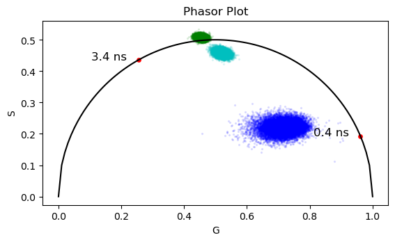
The bound/free NADH is usually related to the oxidative phosphorillation or glycolysis. The conclusion is made based on the position of the transformed data in the phasor plot in relation to the free and bound components.

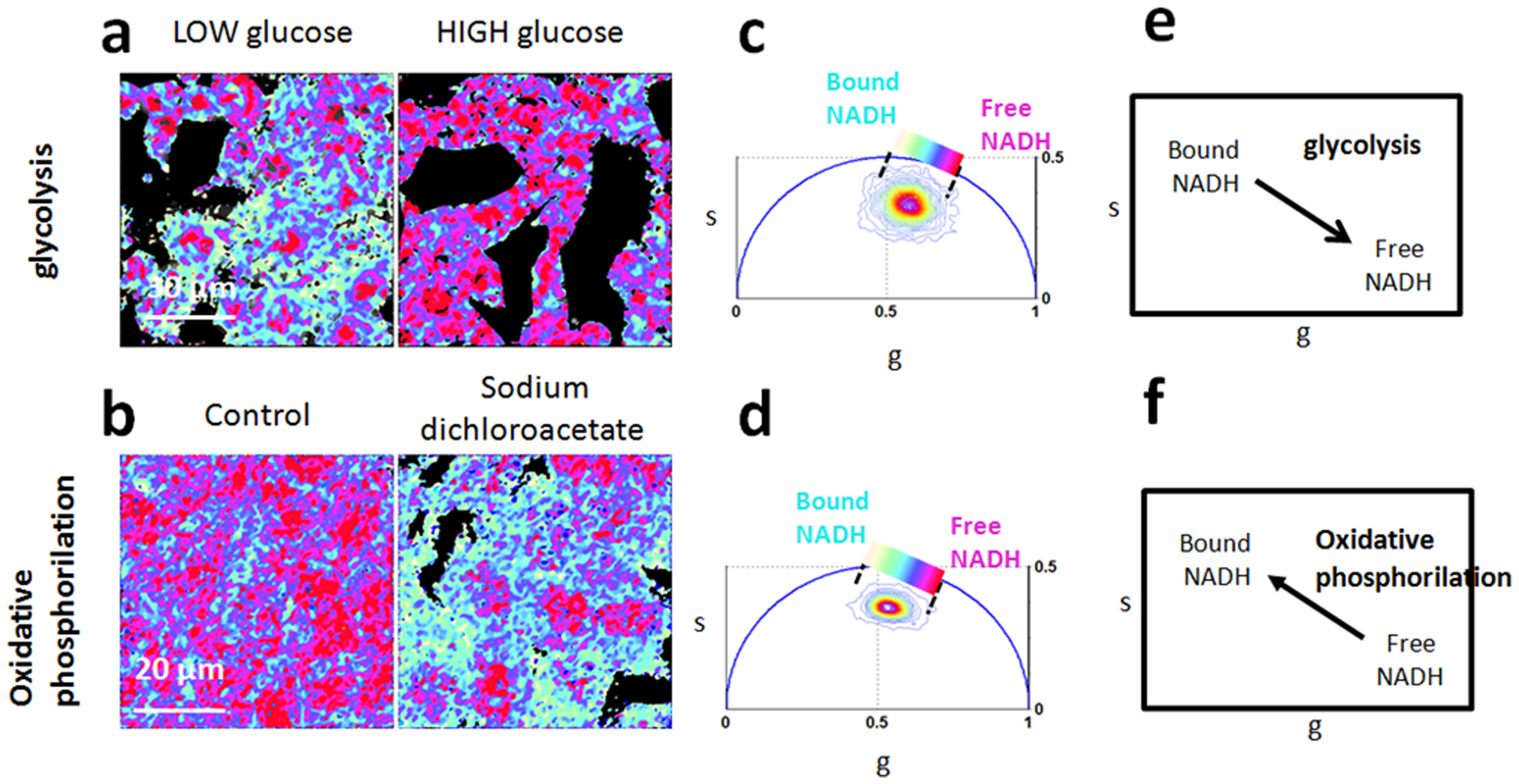
Created by Stringari, C. et al. PLOS ONE, 2012. Phasor Fluorescence Lifetime Microscopy of Free and Protein-Bound NADH Reveals Neural Stem Cell Differentiation Potential

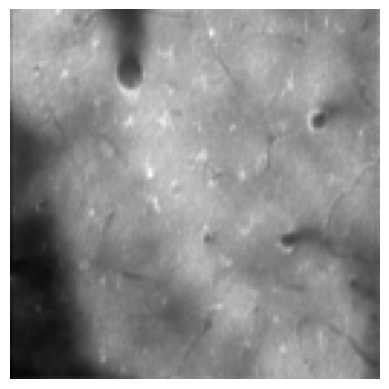
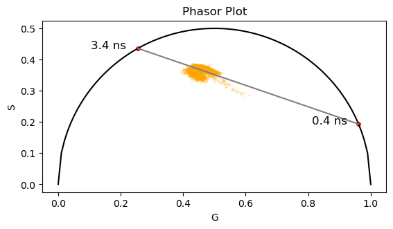
Second, we load the image of the brain cells and display the data in phasor plot:

# Mixture of rhodamineB(10%) and erytrosineB(90%) in methanol
# Load erytrosine B data and plot the monoexponential decay in phasor
# Select the sdt file
file_path = "./static/sdt/240906_mouse_001_non_tumor/1024x1024x256_FLIM_NADH_750nm_472-30.sdt"
# Load the sdt file and print the number of channels
flim_file = SdtFile(file_path)
print("The number of channels is: ", len(flim_file.data))
# Load the data from first channel
data = flim_file.data[0]
print("The shape of the data is (x, y, time bins): ", data.shape)
# Plot the flourescence lifetime decay for a pixel and binned data
# Create a time array for the x-axis
time = np.linspace(0, 12.5, data.shape[2])
# Binned data according to the bin factor and keep the third dimension
data_binned = data.reshape((data.shape[0] // bin_factor, bin_factor,
                            data.shape[1] // bin_factor, bin_factor,
                            data.shape[2])).sum(axis=(1, 3))
# create image to display
intensity_image = np.sum(data_binned, axis=2)

# Calculate the phasor coordinates for all the point in the image
g_cells_all = []
s_cells_all = []

for idx_x in range(data_binned.shape[0]):
    for idx_y in range(data_binned.shape[1]):
        pixel_decay = data_binned[idx_x, idx_y, :]
        # Find the index of the maximum value in decay data
        max_index = np.argmax(pixel_decay)   
        # Slice the vector to keep only the values on the right side behind the peak
        sliced_data = pixel_decay[max_index:]
        sliced_time = time[max_index:]
        sliced_time = sliced_time - sliced_time[0]
        # Time vector
        t = sliced_time*1e-9
        g = np.sum(sliced_data * np.cos(omega * t)) / np.sum(sliced_data)
        s = np.sum(sliced_data * np.sin(omega * t)) / np.sum(sliced_data)
        g_cells_all.append(g)
        s_cells_all.append(s)
# Plot the phasor plot with the NADH points
fig, ax = plt.subplots(1,1)
ax.imshow(intensity_image, cmap='gray')
ax.axis('off')
fig, ax = plt.subplots(1,1)
ax.scatter(g_cells_all, s_cells_all, s = 2, c='orange', alpha=0.1)
ax.plot(x_corr, y_corr, 'k')
ax.plot([g_NADH[0], g_NADH[1]], [s_NADH[0], s_NADH[1]], 'gray')
ax.scatter(g_NADH, s_NADH, s=15, c='r')
ax.set_xlabel('G')
ax.set_ylabel('S')
ax.set_title('Phasor Plot')
# Plot text in x, y coordinates
ax.text(g_NADH[0]-0.15, s_NADH[0], '3.4 ns', color='k', fontsize=12)
ax.text(g_NADH[1]-0.15, s_NADH[1], '0.4 ns', color='k', fontsize=12)
ax.axes.set_aspect('equal') 

The number of channels is:  2
The shape of the data is (x, y, time bins):  (1024, 1024, 256)

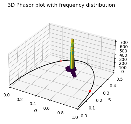
# Create a 2D histogram of the g and s values
hist, xedges, yedges = np.histogram2d(g_cells_all, s_cells_all, bins=50)

# Construct arrays for the anchor positions of the bars.
xpos, ypos = np.meshgrid(xedges[:-1] + 0.01, yedges[:-1] + 0.01, indexing="ij")
xpos = xpos.ravel()
ypos = ypos.ravel()
zpos = 0

# Construct arrays with the dimensions for the bars.
dx = dy = 0.02 * np.ones_like(zpos)
dz = hist.ravel()

# Filter out the zero values
nonzero = dz > 0
xpos = xpos[nonzero]
ypos = ypos[nonzero]
dz = dz[nonzero]

# Create the 3D plot
fig = plt.figure()
ax = fig.add_subplot(111, projection='3d')

# Use a colormap to color the bars based on their height
colors = plt.cm.viridis(dz / max(dz))

ax.bar3d(xpos, ypos, zpos, dx, dy, dz, color=colors, zsort='average')
ax.plot(x_corr, y_corr, 'k')
ax.scatter(g_NADH, s_NADH, s=15, c='r')
ax.set_xlim([0, 1])
ax.set_ylim([0, 0.5])
ax.set_xlabel('G')
ax.set_ylabel('S')
ax.set_zlabel('Frequency')
ax.set_title('3D Phasor plot with frequency distribution')
ax.set_box_aspect([1, 1, 0.5])  # Aspect ratio is 1:1:0.5
plt.show()

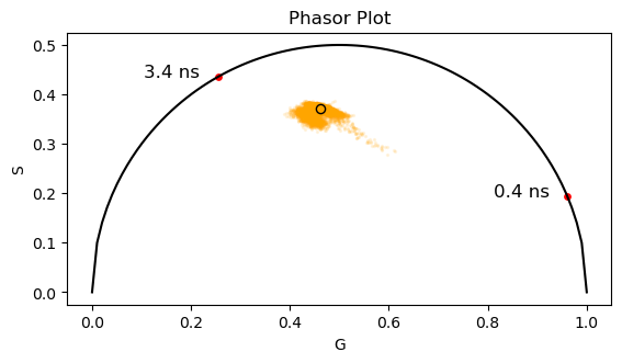
# Calculate the center of mass of the phasor plot
g_center = np.sum(g_cells_all) / len(g_cells_all)
s_center = np.sum(s_cells_all) / len(s_cells_all)

# Plot the phasor plot with the NADH points
fig, ax = plt.subplots(1,1)
ax.scatter(g_cells_all, s_cells_all, s = 2, c='orange', alpha=0.1)
ax.scatter(g_center, s_center, s = 35, c='orange', edgecolors='black')
ax.plot(x_corr, y_corr, 'k')
ax.scatter(g_NADH, s_NADH, s=15, c='r')
ax.set_xlabel('G')
ax.set_ylabel('S')
ax.set_title('Phasor Plot')
# Plot text in x, y coordinates
ax.text(g_NADH[0]-0.15, s_NADH[0], '3.4 ns', color='k', fontsize=12)
ax.text(g_NADH[1]-0.15, s_NADH[1], '0.4 ns', color='k', fontsize=12)
ax.axes.set_aspect('equal') 

# Calculate the ratio of bound NADH
# The quantum yield of bound NADH is 6x higher than free NADH
qy = 6
d_bound = np.sqrt((g_center - g_NADH[0])**2 + (s_center - s_NADH[0])**2)
d_free = np.sqrt((g_center - g_NADH[1])**2 + (s_center - s_NADH[1])**2)
free_nadh_fraction = (d_bound / qy) / ((d_bound / qy) + d_free)
print(f"The ratio of bound NADH is: {free_nadh_fraction*100:.2f}", "%")   

The ratio of bound NADH is: 6.34 %