Fluorescence lifetime microscopy (FLIM)

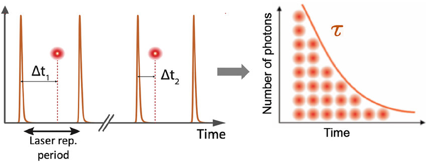
Time correlated single photon counting (TCSPC) detects single photons of a periodic light signal and determines the times of the photons after the excitation pulses.

FLIM theory

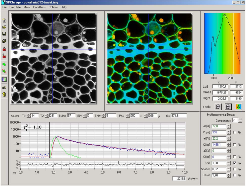
Fitting a model to the decay curve approach

A fluorophore decays with time according to the relation:

\[ I_{(t)} = A_0e^{-t/\tau_0} \]

where \(\tau_0\) is the fluorescence lifetime and \(A_0\) is the amplitude.

To model more complex kinetics of fluorophores, the decay is usually model by a sum of exponentials:

\[ I_{(t)} = \sum_{i=1}^n A_ie^{-t/\tau_i} \]

where \(\tau_0\) is the fluorescence lifetime and \(A_0\) is the amplitude.

The model fit can be done in specialized SW or by scripting.

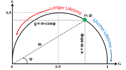
Phasor plot: the model-free approach

Representation of the fluorescence lifetime using the phasor plot model-free aproach. The phasor is a graphical representation of the transformed raw data.

The single decay component fluorophore sits on the universal circle and the position on the circle reflects the lifetime \(\tau_0\) in respect with the laser repetition rate \(\omega\).

The two phasors \(g\) and \(s\) are obtained through the transformation as:

\[ g_{(x,y)}(\omega) = \frac{\int I_{x,y}(t)\cos(\omega t)\,dt\,}{\int I_{x,y}(t)\,dt\,} \]

\[ s_{(x,y)}(\omega) = \frac{\int I_{x,y}(t)\sin(\omega t)\,dt\,}{\int I_{x,y}(t)\,dt\,} \]

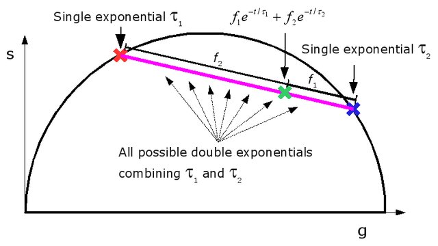
The graphic represantation of the phasor is the universal semicircle with a point cloud of transformed decayes.

The complex micture of fluorescence specimen will be represented as a linear combination of those specimen in the universal semicircle.

Code blocks for FLIM data phasor analysis

The B&H FLIM data can be analysed in Python using multiple libraries such as numpy, sdtfile and others. The practical examples are on the next pages.